Felix Immanuel

An Engineer with 6+ years of experience as a Business Analyst. Adept in EDA and Machine Learning. Has a sound knowledge of Agile and Scrum.
View My LinkedIn Profile
Adult Dataset & their Income Analysis
Project description:
The “Adult Dataset has around 32,000 records with various information like age, education, marital-status, occupation, gender, hours per week, country and income information”. From this dataset I have derived various insights and explained them below.
1. Dataset Overview
adt=pd.read_csv('adult.csv')
adt.head()

    age         workclass  fnlwgt  ... hours-per-week  native-country income
0   39         State-gov   77516  ...             40   United-States  <=50K
1   50  Self-emp-not-inc   83311  ...             13   United-States  <=50K
2   38           Private  215646  ...             40   United-States  <=50K
3   53           Private  234721  ...             40   United-States  <=50K
4   28           Private  338409  ...             40            Cuba  <=50K
2. Checking for NULL values in the data
adt.isnull().sum()

age               0
workclass         0
fnlwgt            0
education         0
education-num     0
marital-status    0
occupation        0
relationship      0
race              0
sex               0
capital-gain      0
capital-loss      0
hours-per-week    0
native-country    0
income            0
No Null values in this dataset.
3. Changing the column Names
Existing Column Values: Index([‘age’, ‘workclass’, ‘fnlwgt’, ‘education’, ‘education-num’, ‘marital-status’, ‘occupation’, ‘relationship’, ‘race’, ‘sex’, capital-gain’, ‘capital-loss’, ‘hours-per-week’, ‘native-country’, ‘income’],dtype=’object’)
adt.rename(columns={'marital-status' : 'marital'}, inplace = True)
adt.rename(columns={'capital-gain' : 'capgain'}, inplace = True)
adt.rename(columns={'capital-loss' : 'caploss'}, inplace = True)
adt.rename(columns={'hours-per-week' : 'hrsprwk'}, inplace = True)
adt.rename(columns={'native-country' : 'country'}, inplace = True)
Corrected Column Values: Index([‘age’, ‘workclass’, ‘fnlwgt’, ‘education’, ‘education-num’, ‘marital’, ‘occupation’, ‘relationship’, ‘race’, ‘sex’, ‘capgain’, ‘caploss’, ‘hrsprwk’, ‘country’, ‘income’], dtype=’object’)
4. Grouping the “Countries” into Region
There were 42 unique entries in the country column and around 583 entries where unknow.
adt['country'].value_counts()

United-States                 29170
Mexico                          643
?                               583
Philippines                     198
Germany                         137
Canada                          121
Puerto-Rico                     114
El-Salvador                     106
India                           100
Cuba                             95
England                          90
Jamaica                          81
South                            80
China                            75
Italy                            73
Dominican-Republic               70
Vietnam                          67
Guatemala                        64
Japan                            62
Poland                           60
Columbia                         59
Taiwan                           51
Haiti                            44
Iran                             43
Portugal                         37
Nicaragua                        34
Peru                             31
Greece                           29
France                           29
Ecuador                          28
Ireland                          24
Hong                             20
Trinadad&Tobago                  19
Cambodia                         19
Thailand                         18
Laos                             18
Yugoslavia                       16
Outlying-US(Guam-USVI-etc)       14
Hungary                          13
Honduras                         13
Scotland                         12
Holand-Netherlands                1
Name: country, dtype: int64
Grouping all the countries into 4 regions (America, Asia, Europe, Others).
Creating a new column
adt['region']='Asia'
Grouping the countries
adt['region'][adt['country'].isin(['United-States','Canada','Mexico','Puerto-Rico','El-Salvador','Jamaica','Guatemala','Columbia',
    'Nicaragua','Trinadad&Tobago','Cambodia','Laos','Outlying-US(Guam-USVI-etc)','Honduras'])]='America'

adt['region'][adt['country'].isin(['Germany','England','Italy','Dominican-Republic','Poland','Iran','Portugal','France','Greece',
    'Ecuador','Ireland','Scotland','Holand-Netherlands'])]='Europe'

adt['region'][adt['country'].isin(['?',])]='Others'
Region Overview
adt['region'].value_counts()

America    30475
Asia         870
Europe       633
Others       583
Name: region, dtype: int64
5. Grouping the “Education Entries” into Categories
There were 16 unique entries in the education column.
adt['education'].value_counts()

HS-grad         10501
Some-college     7291
Bachelors        5355
Masters          1723
Assoc-voc        1382
11th             1175
Assoc-acdm       1067
10th              933
7th-8th           646
Prof-school       576
9th               514
12th              433
Doctorate         413
5th-6th           333
1st-4th           168
Preschool          51
Name: education, dtype: int64
Grouping all the education into 3 categories (School, Graduate, Other Education)
adt['edu_category']='School'
adt['edu_category'][adt['education'].isin(['HS-grad','Some-college','Bachelors','Masters','Doctorate'])]='Graduate'
adt['edu_category'][adt['education'].isin(['Assoc-voc','Assoc-acdm'])]='OthrEDU'
Education Category Overview
adt['edu_category'].value_counts()

Graduate    25283
School       4829
OthrEDU      2449
Name: edu, dtype: int64
6. Grouping the “Occupation” into Job Categories
There were 15 unique entries in the occupation column.
adt['occupation'].value_counts()

Prof-specialty       4140
Craft-repair         4099
Exec-managerial      4066
Adm-clerical         3770
Sales                3650
Other-service        3295
Machine-op-inspct    2002
?                    1843
Transport-moving     1597
Handlers-cleaners    1370
Farming-fishing       994
Tech-support          928
Protective-serv       649
Priv-house-serv       149
Armed-Forces            9
Name: occupation, dtype: int64
Grouping all the occupation into 2 categories (officeJobs, fieldJobs)
adt['jobCategory']='officeJobs'
adt['jobCategory'][adt['occupation'].isin(['Craft-repair','Sales','Transport-moving','Handlers-cleaners','Farming-fishing'])]='fieldJobs'
Job Category Overview
adt['jobCategory'].value_counts()

officeJobs    20851
fieldJobs     11710
Name: occu, dtype: int64
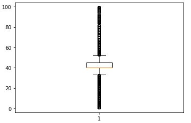
7. Processing “Hours-per-week” Column
Checking for Outliers in the “Hours-per-week” Column.
plt.boxplot(adt['hrsprwk'])
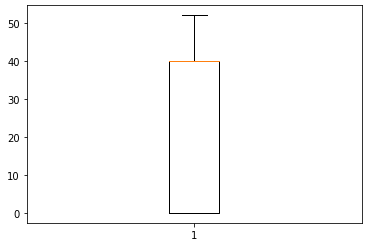
Treating the Outliers
p25=adt['hrsprwk'].quantile(.25)
p75=adt['hrsprwk'].quantile(.75)

iqr=p75-p25

lowerrange=p25-(1.5*iqr)
upperrange=p75+(1.5*iqr)

adt['hrsprwk'][adt['hrsprwk']<lowerrange]=np.nan
adt['hrsprwk'][adt['hrsprwk']>upperrange]=np.nan

adt['hrsprwk'].isnull().sum()
adt['hrsprwk'].fillna(0,inplace=True)
After treating the Outliers.
plt.boxplot(adt['hrsprwk'])
8. Getting Dummies from the newly created column for “Random Forest ML Algorithm”
Getting dummies for “Region”.
r=pd.get_dummies(adt['region'])
adt=pd.concat([adt,r], axis=1)
Getting dummies for “Gender”.
s=pd.get_dummies(adt['sex'])
adt=pd.concat([adt,s], axis=1)
Getting dummies for “Education Category”.
e=pd.get_dummies(adt['edu_category'])
adt=pd.concat([adt,e],axis=1)
Getting dummies for “Gender Category”.
o=pd.get_dummies(adt['jobCategory'])
adt=pd.concat([adt,o],axis=1)
Getting dummies for “Workclass”.
wk=pd.get_dummies(adt['workclass'])
adt=pd.concat([adt,wk],axis=1)
Getting dummies for “Marital Status”.
ma=pd.get_dummies(adt['marital'])
adt=pd.concat([adt,ma],axis=1)
Getting dummies for “Family Relationship Status”.
re=pd.get_dummies(adt['relationship'])
adt=pd.concat([adt,re],axis=1)
Columns list before getting dummies
adt.columns

Index(['age', 'workclass', 'fnlwgt', 'education', 'education-num', 'marital', 'occupation', 'relationship', 'race', 'sex', 'capgain', 'caploss', 'hrsprwk', 'country', 'income'], dtype='object')
Columns list after getting dummies
adt.columns
Index(['age', 'workclass', 'fnlwgt', 'education', 'education-num', 'marital', 'occupation', 'relationship', 'race', 'sex', 'capgain', 'caploss', 'hrsprwk', 'country', 'income', 'region', 'Female', 'Male', 'edu', 'occu', 'Graduate', 'OthrEDU', 'school', 'fieldJobs', 'officeJobs', 'America', 'Europe', 'Others', 'asia', 'Federal-gov', 'Local-gov', 'Never-worked', 'Private', 'Self-emp-inc', 'Self-emp-not-inc', 'State-gov', 'Without-pay', 'Divorced', 'Married-AF-spouse', 'Married-civ-spouse', 'Married-spouse-absent', 'Never-married',
'Separated', 'Widowed', 'Husband', 'Not-in-family', 'Other-relative', 'Own-child', 'Unmarried', 'Wife'], dtype='object')
9. Dataset Insights
The below insights are about the people who earn more according to each category.
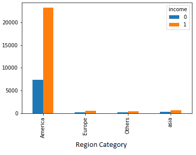
1. Income comparison according to a “Region”
People who lives in the American region earns more than any other people in the world.
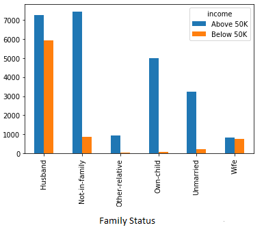
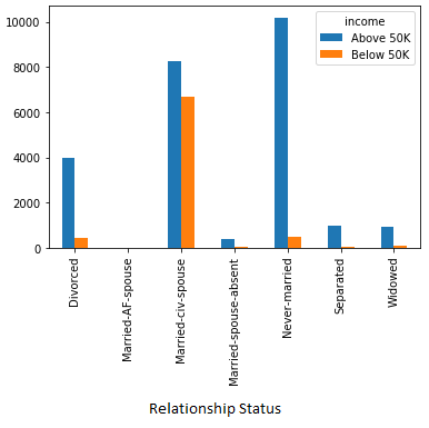
2. Income comparison of an individual according to his “Family Status”
The Person who is not in a family earns more money than any other category and in a family Husbands earn more than all.
3. Income comparison according to an individuals “Marital Status”
People who is not married earns more than any other marital status.
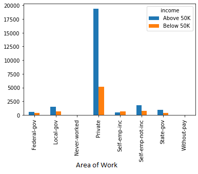
4. Income comparison according to the “Job Sector”
People who work in the private sector earns more than the people who works in the government & other areas.
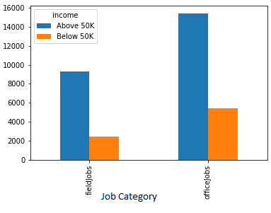
5. Income comparison as per “Job”
People who are working in professional office jobs earn more than the people who work in field jobs.
6. Income comparison as per the “Education”
Graduates earn more than the people who didn’t complete graduation.

10. Building Model (Random Forest ML Algorithm)
1. Importing the dataset
X = adt[['Female','America','Europe','asia','Federal-gov', 'Local-gov', 'Never-worked', 'Private', 'Self-emp-inc', 'Self-emp-not-inc', 'State-gov', 'Divorced', 'Married-AF-spouse', 'Married-civ-spouse', 'Married-spouse-absent', 'Never-married', 'Separated','Husband', 'Not-in-family', 'Other-relative', 'Own-child', 'Unmarried']]

y = adt[['income']]
2. Splitting the dataset into the Training set and Test set
from sklearn.model_selection import train_test_split
X_train, X_test, y_train, y_test = train_test_split(X, y, test_size = 0.25, random_state = 0)
3. Fitting Random Forest to the Training set
from sklearn.ensemble import RandomForestClassifier
classifier=RandomForestClassifier()
classifier.fit(X_train,y_train)
4. Predicting the Test set results
y_pred = classifier.predict(X_test)
5. Prediction Accuracy
print("The train accuracy " , classifier.score(X_train,y_train)*100)
print("The test accuracy " , classifier.score(X_test,y_test)*100)
The train accuracy 98.29
The test accuracy 81.88